
In mathematics, computer science, and operations research, Optimization simply means picking the absolute best element from a set of available alternatives. Whether you are an electricity provider figuring out how many power plants to build, or a warehouse manager trying to shorten the distance your workers walk, you are trying to optimize.
But how do computers and mathematicians do this? Let’s break down the basic language of optimization.
The Holy Grail: Convexity
If you talk to anyone who works in optimization, you will hear the word “Convex” a lot. Convexity is a highly desired property for a cost function (the mathematical formula of the thing we want to minimize, like cost or distance).
Why? Because if a problem is convex, it guarantees that finding a “good” solution means you have actually found the best possible solution.
Let’s look at what this means visually:
1. Convex Sets
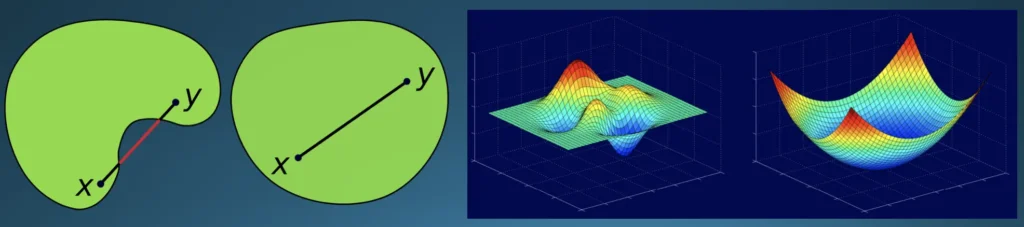
Imagine a shape. If you can pick any two points inside that shape, draw a straight line between them, and that entire line stays inside the shape, it is a Convex Set.
- Look at the first green circle in the image above. Any line drawn between two points stays inside. It’s convex.
- Look at the second green shape (the one with a “bite” taken out of it). If you draw a line across the “bite,” the line travels entirely outside the shape. It is not convex.
2. Convex Functions
Now let’s apply this to a graph. Imagine a curve that looks like a smooth bowl (like the second 3D graph in the image above).
A function is convex if you pick any two points on its graph, draw a straight line connecting them, and the straight line hovers above or exactly on the curve.
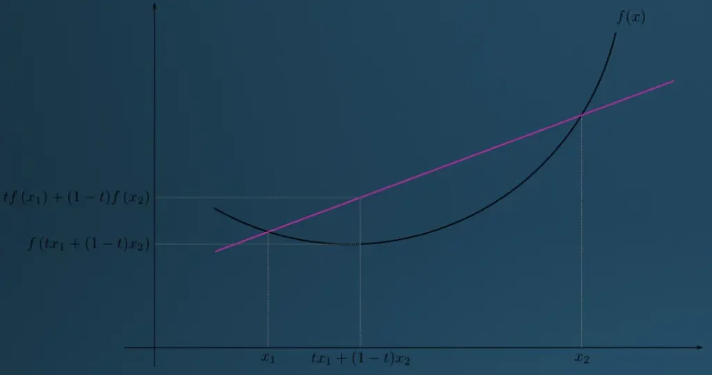
Mathematicians write this rule using this formula:
f(tx_1 + (1-t)x_2) \leq tf(x_1) + (1-t)f(x_2)
Don’t let formula scares you. and is just random points in x-axis, and is just another point that guaranteed to be in between and (if , it is ; if , it is ; if , it is right on the middle)
This formula simply says: “The actual curve of the graph () is always sitting lower than the straight line drawn between two points on the graph.”
3. Strictly Convex
If we want to be even more rigid, we have Strictly Convex functions. This just means the straight line sits strictly above the graph and never touches it at all, except exactly at the starting and ending dots.
The math looks almost identical, but we replace the “less than or equal to” () with a strict “less than” ():
f(tx_1 + (1-t)x_2) < tf(x_1) + (1-t)f(x_2)
The Flavours of Optimization
Optimization isn’t a one-size-fits-all tool. Problems come in different flavors depending on what you are trying to solve in the real world. Let’s look at the four main comparisons:
1. Continuous vs. Discrete
- Continuous Optimization: Your variables can be any real number (). For example, if you are mixing chemicals, you could use exactly 2.718 liters. The numbers flow continuously.
- Discrete (Integer) Optimization: Sometimes, fractions don’t make sense. If an electricity provider is planning to build power plants over the next 5 years, they can’t build 2.5 power plants. They must build 2 or 3. Because the variables can only be whole integers, this is called an integer programming problem.
2. Unconstrained vs. Constrained
- Unconstrained: There are no rules or limits on your variables. You can do whatever you want to find the absolute maximum or minimum.
- Constrained: You have strict limits (constraints), which can be linear, nonlinear, or convex. (Think of our suitcase analogy: the bag must weigh less than 50 lbs).
- Pro-Tip: Constrained problems are much harder for computers to solve. To fix this, mathematicians often “smuggle” the constraints directly into the cost function to trick the computer into solving it like an easier, unconstrained problem.
3. Deterministic vs. Stochastic
- Deterministic: There are no surprises. Every parameter is known. For example, if you are optimizing a warehouse layout to minimize worker walking distance, the distance between shelves won’t suddenly change.
- Stochastic: The world is random, and you don’t have all the facts. If you are optimizing a financial portfolio, stock returns go up and down based on unpredictable market conditions. Stochastic programming tackles this uncertainty to find the best solution “on average.”
4. Local vs. Global
Imagine you are blindfolded in a mountain range, trying to find the lowest valley.
- Local Optimization: You feel the ground with your feet and walk downward until you hit a flat bottom. You found a valley. But is it the lowest valley in the whole mountain range? You don’t know. You only found the best solution in your local area. Many algorithms only seek local solutions.
- Global Optimization: This is the absolute best solution everywhere. Finding it is incredibly difficult.
If your cost function, your constraints, and your variables are all convex, a magical mathematical property happens: Any local optimum is guaranteed to be the unique global optimum.
If you drop a marble into a perfect bowl (a convex shape), it rolls perfectly to the single lowest point at the bottom. There are no fake valleys to get trapped in.
Unfortunately, while perfectly smooth, convex bowls are a mathematician’s dream, most real-world problems are beautifully messy—they are highly constrained, non-convex, and often stochastic. In real life, you almost never have unlimited resources; your budget runs out, time is finite, and physical materials are limited, which makes practically every real problem a constrained one.
Furthermore, the real world is full of unpredictable surprises like fluctuating stock prices or sudden weather changes (stochastic), and it often forces you to make whole-number choices, like deciding to buy exactly 3 trucks instead of 2.5 (discrete). Because of these rigid limits, jumpy integer variables, and unpredictable variables, real-world graphs rarely look like smooth bowls; instead, they look like jagged, multi-peaked mountain ranges (non-convex), making the hunt for that single, perfect “global” solution one of the most difficult and exciting challenges in computer science.