2.2 Prices and Returns

The price of an asset is the most obvious quantity in financial markets. Denoted by $p_t.$ For future references:

 y_t \overset{\triangle}{=} \log p_t 

So why do we take logarithm of raw price? Because raw prices doesn’t show the percentage, where we care about percentage

For example, We have two stocks with A=10$ and B=100$. If both stocks go up by 10$ and if you graph both of them, you see that lines go up equally, but in reality stock A just doubled, while stock B only go up by %10, which is 5 times lower.

So, the simplest model for the log prices is the random walk:

 y_t = \mu + y_{t-1} + \epsilon_t 

• $y_t$: Log price of exactly now.
• $\mu$ (drift): Our reward. Generally indicates slow, upward movement of stock market. Could be negative. Our model predicts it.
• $y_{t-1}$: Log price of time minus one step backward.
• $\epsilon_t$: Random noise of market at now.

We don’t try to estimate the $\epsilon_t$, instead we estimate how big the noise will be. The $\mu$ values are also depends on the frequency you interested in. And the all trick is is basically data modeling. Once you get $\mu$ and $\sum$, anyone can use portfolio optimisation, basically all you have to do is to find $\mu$ and $\sum$ as best as you can.

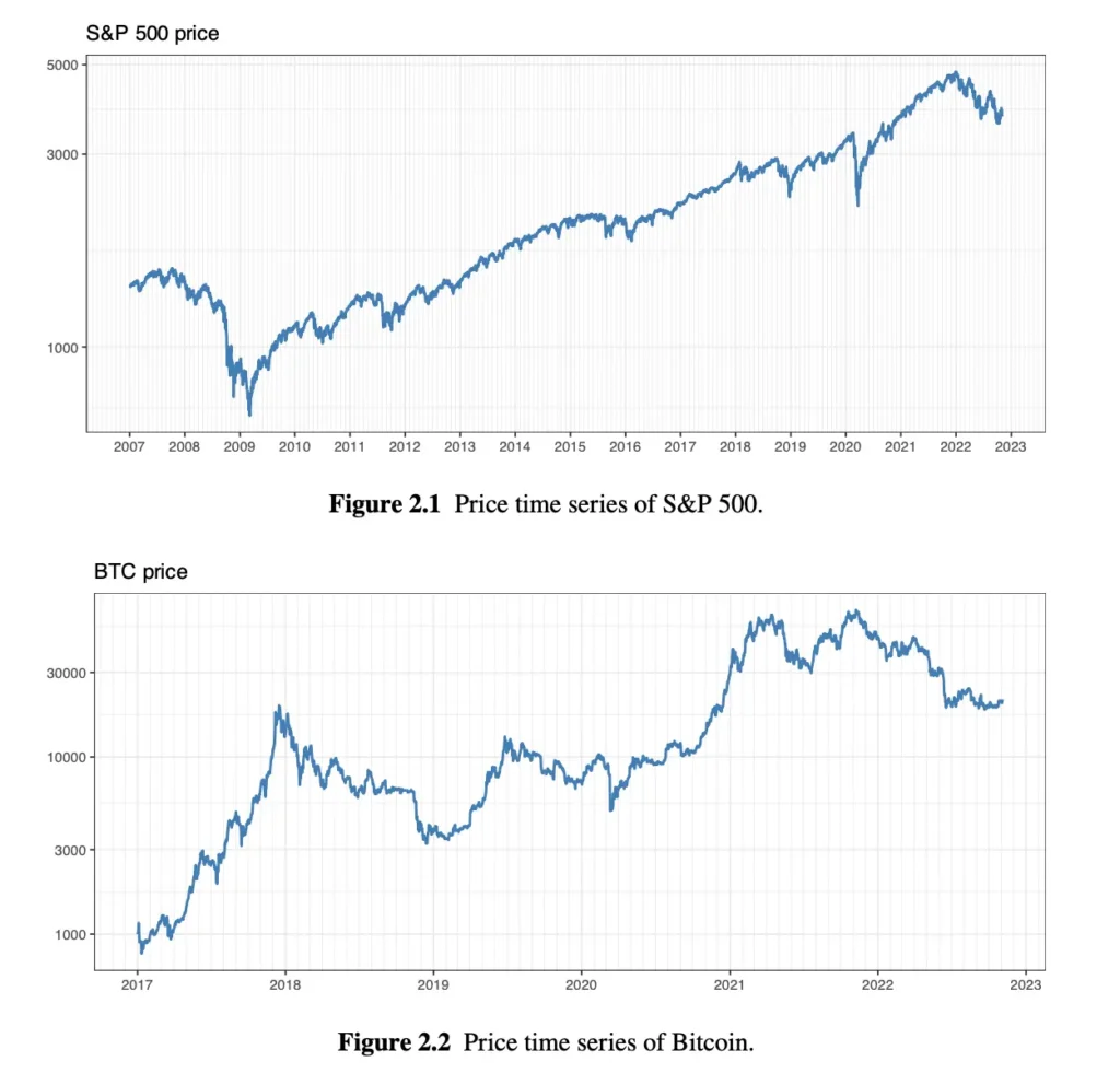
Above graphs represents the log prices of S&P and Bitcoin over time, which is basically a time series of their prices.

As we say, we are not dealing with prices of stocks because when you look at it, they always go upwards (Apple went from $1 to $150 over twenty years), so modeling these are not good for computers. Instead, we convert these prices into daily percentages (returns), then we have stable heartbeat bouncing around zero (+1%, -2%, +0.5%, +1.2%). This behavior is called stationarity, and statistical models love these.

So how do we calculate returns? There are 2 basic ways to calculate return:

1. The Linear (Simple) Return: It is basic percentage change.

 r_t^{lin} \overset{\triangle}{=} \frac{p_{t} - p_{t-1}}{p_{t-1}} = \frac{p_t}{p_t-1} - 1 

• $r_t^{lin}$: The linear return (r) of today (t).
• $p_t$: The price of today (raw price, not log price).
• $p_{t-1}$: The price of yesterday.

For example, we bought a stock yesterday for 100$, today it is worth 110$. $(110-100)/100 = 0.1 = +\%10$ return.

Linear returns are additive among assets. Means that when we have a portfolio among different assets, using linear return makes calculating total profit easy. For example we split our money to 2 assets equally, stock A goes up %10, stock B goes down %4, so total return is $(0.5 \times \%10) + (0.5 \times -\%4) = \%3$ total portfolio return.

2. The Log (continuously compounded) return: 

 r_t^{log} \overset{\triangle}{=} y_t - y_{t-1} = \log(\frac{p_t}{p_{t-1}}) 

Log returns are additive along the time domain. Means that if we want to know how much a stock returned over a month, we just add up 30 days of daily log returns. This is why log returns are favourite tool for data modeling.

Since we use log prices, the difference between them is basically $\mu$, we no longer care if Apple is a $150 stock or a $300 stock. It only sees a flat, stable heartbeat of percentage changes:

 r_t^{log} \overset{\triangle}{=} y_t - y_{t-1} = \mu + \epsilon_t 

This is the “stationary” concept that we have talked about.

We can easily convert log return into linear return (or vica versa) through simple formula:

 r_t^{log} = \log(1 + r_t^{lin}) 

• If a stocks daily return is small (like $r_t^{log} \approx r_t^{lin}$ 5), then $r_t^{log} \approx r_t^{lin}$.

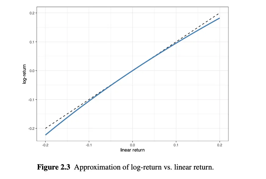
Look at the Figure 2.3, between -0.05 and +0.05 log return and linear return almost the same, but when the difference increases, we can no longer just swap them.

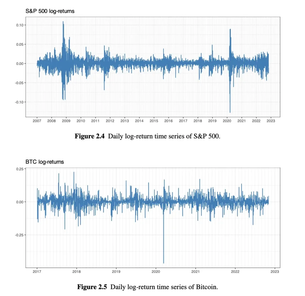
Figure 2.4 shows the daily log-returns of the S&P stock index over a span of more than a decade. One can easily observe the high-volatility period during the global financial crisis in 2008, as well as the high peak in volatility in early 2020 due to the COVID-19 pandemic.

Figure 2.5 shows the daily log-returns of Bitcoin over six years. Observe the Bitcoin flash crash on March 12, 2020, with a drop close to 50% in a single day.

Look at the numbers. S&P limits are -0.1 and +0.1, whereas Bitcoin’s limits are -0.25 and +0.25, means that Bitcoin have higher volatility

In general sense, we annualise the volatility of stocks, then if resulting value is between %12 and %20, volatility is considered low. If value is above %30, it considered as extremely volatile.

So how do we calculate annualised data from volatility data? Assume that we have daily frequency:

1. Find daily volatility (daily $\sigma$): How values spikes from 0.0 daily? For S&P 500, it is roughly %1.3, for Bitcoin, it is roughly %4.1.
2. To find yearly risk, we cannot simply multiply the value with 365 because graphs follows random walk, if one day it goes up by %1 and another day goes down %1, they cancel each out. To calculate yearly risk, we use square root of time

 \text{Annualized Volatility} = \text{Daily Volatility } \times \sqrt{\text{Num of Trading Days in a Year}} \\ 
  \text{S\&P 500 Volatility} = \%1.3 \times \sqrt{252} = \%1.3 \times 15.87 = \%20.6  \\
  \text{Bitcoin Volatility} = \%4.1 \times \sqrt{365} = \%4.1 \times 19.1 = \%78.3 

• (The stock market is not open on weekends and holidays, whereas crypto never sleeps).

Resources

Portfolio Optimisation: Theory and Application by Daniel P. Palomar, Page 20, 21, 22, 23.