Introduction

Modern portfolio theory started with Harry Markowitz. His idea is that risk-averse investors should optimize their portfolio based on a combination of two objectives:

• Expected return
• Risk.

In Pre-Markowitz era, investors also looked at expected return and risk, but instead of considering overall portfolio, they considered every single stock in isolation, Markowitz changed this by looking at the overall portfolio.

Today, since Markowitz formulation does not perform as anticipated, most people use it with various heuristics or just refrain from using it.

Random Variable X: Something whose exact outcome we don’t know yet. Future return of a stock

Mean $\mu$ and Expected value $\mathbf{E}[]$: The average long-term result of something. For example if you roll a die millions of times, the $\mathbf{E}[die]=3.5$ ($\mu = \mathbf{E}[]$)

Variance $\sigma^2 = \mathbf{E}[(X – \mu)^2]$: Measures how wildly things swing away from the average. Square it to eliminate negative numbers, then find the average through expected value.

When we are investing, we want high rewards ($\mu$) and low risk ($\sigma$). So to formulate it, we have sharp ratio:

 \text{Sharp Ratio: } \frac{\mu}{\sigma}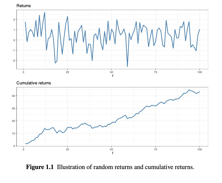 

• In Figure 1.1, the top chart represents the risk ($\sigma$), shows the profit and loss. The bottom chart represents reward ($\mu$), shows what happens to our actual money.
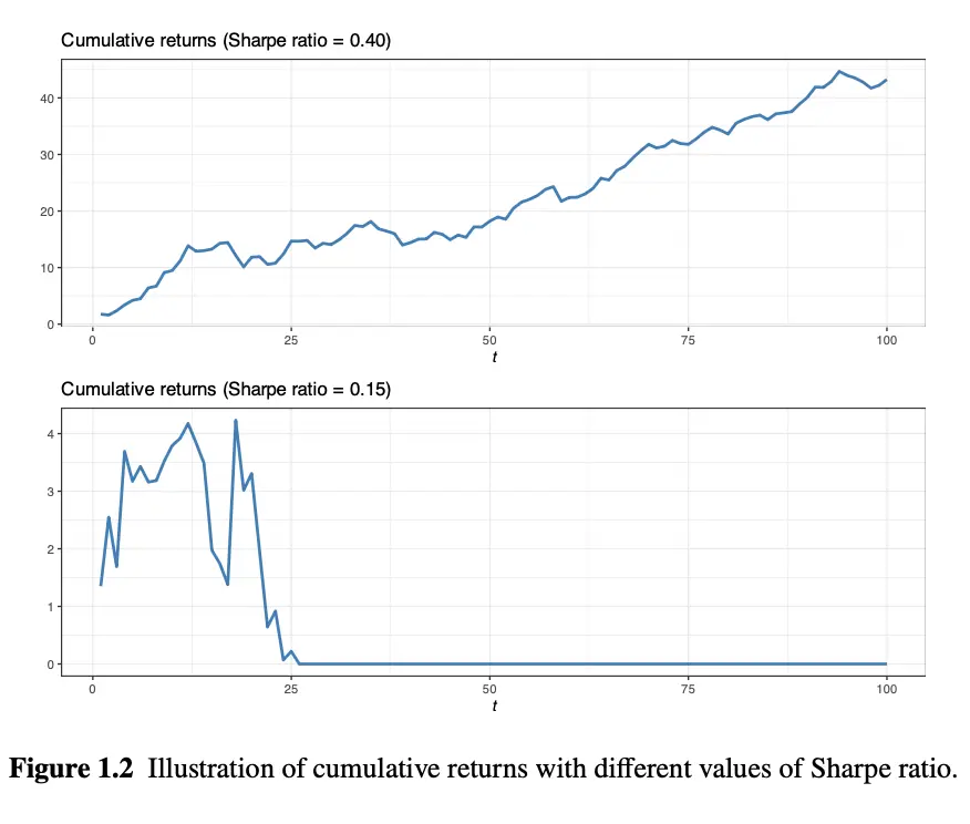
• In Figure 1.2, those two charts shows what we talked earlier. When sharp ratio is high, we profit; When sharp ratio is low, we lose (eventually, bankruptcy).

So what we can do to improve cumulative return (sharp ratio)? Of course random factors cannot be changed, but at least two dimensions can be exploited:

• Temporal Dimension: We know that $X_t$ changes over time, leading time-varying $\mu_t$and $\sigma^2_t$. So we need to adapt the size of the investment to the current value of sharp ratio $\mu_t$ / $\sigma_t$. To predict the sharp ratio at time t, we need a time series model.
• Asset Dimension: We can choose N potential assets with returns $X_1, X_2 \cdots X_N$. If we assume that all of them are independent and identically distributed ($X \sim N(\mu, \sigma^2$))(have same $\mu$ and $\sigma^2$), then the $\mu$ is preserved

 \frac{1}{N}\sum^N_{i=1}X_i 

but our risk is divided by the number of stocks we bought.

 \frac{\sigma^2}{N} 

In reality, we cannot achieve the factor $1/N$ because the random returns $X_i$ are correlated among the assets. They are dependent. So blindly putting equal amounts of money into everything isn’t good enough to protect us. Therefore, engineers have to use math to figure out exactly how much money to put into which specific stocks to dodge that correlation and minimize the total risk. This is called portfolio optimisation (portfolio correlation/portfolio allecation).