2.4 Temporal Structure

The other question is: is the stock market a completely random casino, or are there hidden patterns we can predict?, in math jargon terms:

• i.i.d. (Independent and Identically Distributed): This is math jargon for a perfect coin flip. “Independent” means yesterday’s flip has zero effect on today’s flip. If the market is i.i.d., predicting the future is literally mathematically impossible.
• Temporal Structure: This means hidden patterns over time. Think of the weather: if it rains today, there is a higher statistical probability it will be cloudy tomorrow. Yesterday does affect today.

If the market is i.i.d., then we would have no Machine #1 to predict future $\mu$ and $\sigma$.

Academics in the 1970s studied the market and created a rule called the Efficient-Market Hypothesis (EMH). EMH states that the stock market is a perfectly efficient, all-knowing machine. The second a piece of news happens anywhere in the world, computers instantly buy or sell the stock until it reaches its absolute perfect, fair price.

According to EMH, if every stock is perfectly priced at all times, then “bargains” do not exist. You cannot buy an undervalued stock. Therefore, it is impossible to beat the market. According to EMH, the only possible way to make more money is to buy a riskier asset (like moving from Apple to Bitcoin).

$\alpha$: Alpha is the holy grail. It means “Risk-Adjusted Excess Return.” In plain English, Alpha means beating the market using sheer skill, without taking on extra risk. EMH says Alpha does not exist. It says anyone who beats the market just got lucky, like a guy winning at roulette.

Wall Street practitioners think that EMH is garbage, because people like Warren Buffet and Jim Simons (and its team) found that hidden temporal structures for decades.

If you believe in EMH, there is no need you to read these stuff.

So, let’s try to test the “using past data to to predict future” on computer. We have two acronyms: Autocorrelation Function (ACF) and Partial Autocorrelation Function (PACP).

• “Correlation” means two different stocks moving together (like Apple and Microsoft).
• “Autocorrelation” means a stock moving in sync with its own past ghost.

If autocorrelation exists, then EMH is thrash.

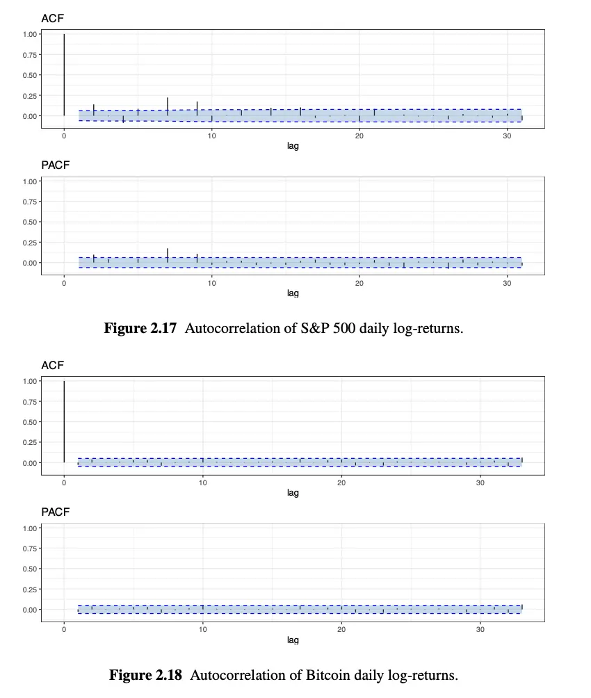
Let’s try to understand the graphs first:

• X-Axis (Lag): This is the number of days in the past. Lag 1 is yesterday. Lag 10 is ten days ago. (Lag 0 is today, which is why there is always a giant spike at 0—today is obviously a 100% perfect copy of today).
• Y-Axis: How strong the copycat effect is.
• The Blue Dashed Band: This is the “Zone of Random Noise.” This is the most important part of the chart. If the little black spikes stay inside this blue band, it means any connection is purely random chance. If a spike pokes out of the blue band, it means you have found a mathematically guaranteed, predictable pattern.

If we look at the charts, we clearly see that almost no black line poke out from blue area, so EMH theory should be correct. but, that would be wrong conclusion. It is true that we cannot predict the direction of the market (up or down), it is linear. But we can predict the mood of the market (calm or crazy), that is non-linear. Here comes the volatility clustering (volatility envelope) term we talked before in stylised facts:

• If the market is having a boring, flat day today… tomorrow will probably be a boring, flat day.
• If the market crashes 5% today… tomorrow will probably feature a massive, violent swing (either up or down).

How do we use this information? We use algorithms to detect when the market’s “mood” is switching from calm to crazy. When the computer detects that a massive storm of volatility is brewing (nonlinear structure), it tells the Optimizer to immediately sell riskier assets and buy safer ones to survive the storm.

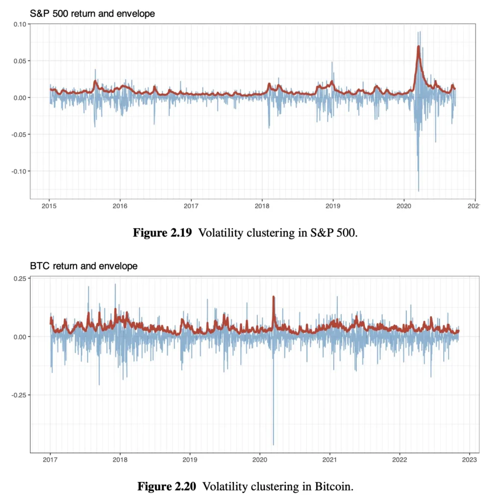
In graph, blue line represents the daily returns (up/down), as we know it looks chaotic. Red line is drawn to trace top of the blue line. Even though blue line is chaotic and unpredictable, red line is smooth and predictable. So how do we prove that we can predict the red line?

The Problem with the old test is that it measured Direction (+ or -). If the market went up +2% today, and down -2% tomorrow, the math said they canceled each other out to zero (random). The quants tell the computer to take the Absolute Value of the returns. So computers stop looking at the direction and considers magnitude.

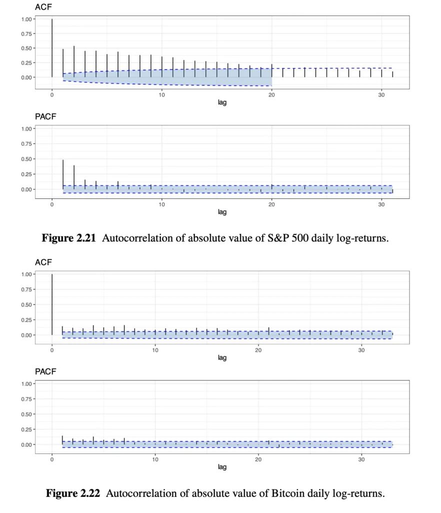
This is the graphs we get when we use absolute values. Black lines almost completely poke out from blue area, means that we have found our hidden temporal structure. Volatility is a massive copycat.

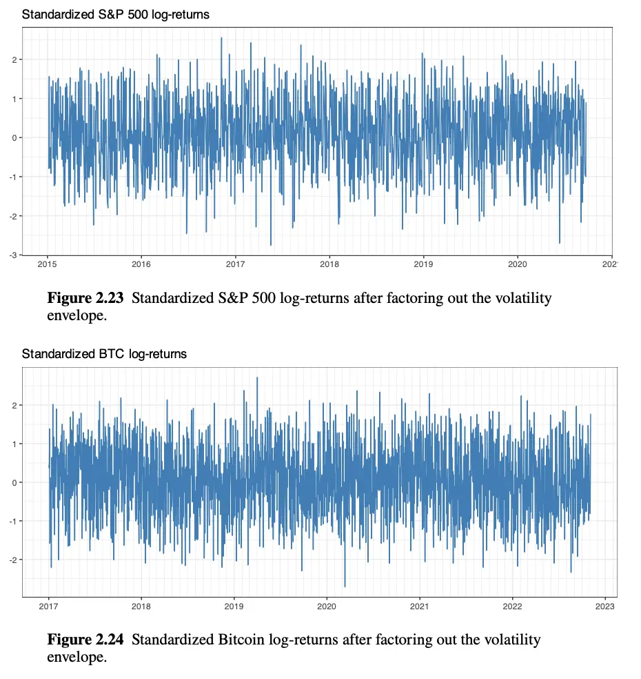
These two charts show what happens if you take the raw, chaotic stock market returns and divide them by that red line that we talked about previously.

• Look at the COVID crash of March 2020 on the S&P 500 chart. It’s gone.
• Because the quant’s computer perfectly predicted that massive volatility was happening, it mathematically filtered it out.
• What left is Standardized Returns. It looks like a perfectly even, boring, uniform block of static noise.

This proves that if a quant builds a good Machine #1, they can mathematically strip away the Black Swans and volatility clustering, leaving behind neat, tidy data that the Markowitz Optimizer can safely digest.

We have proven that “technical analysis” is mostly garbage.

Some might say that: If inflation, interest rates, and earnings all determine the price of a stock, then the stock’s price is the ultimate “summary score.” Why spend 100 hours researching satellite imagery and inflation data and all other things when you can just look at the price? The price already contains all that information!

This is correct, in theory. But in practice, it does not work like this:

• The “Signal vs. Noise” Problem: Imagine Apple stock suddenly drops -3%. If we only look only the prices, all we know is “Apple went down”, we don’t know why
  • Scenario A (Fundamental): Apple’s new iPhone caught on fire, and sales are plummeting. The company is in trouble.
  • Scenario B (Random Noise / $\epsilon_t$): A billionaire CEO got divorced, and his lawyers forced him to sell 10 million shares of Apple today to pay his ex-wife. The company is completely fine.

If we only use past price data (Machine #1), our computer will look at the -3% drop and say, “Apple is going down, sell!”. But if we use fundamental data, our computer will say, “Wait, iPhone sales are great, this price drop is just a billionaire getting divorced. This is a rare discount. BUY!”

Price tells us what happened. Fundamentals tell why it happened. And we need the “why” to predict the future.

Another problem would be speed. Let’s say the Federal Reserve unexpectedly cuts interest rates. That is a massive fundamental event. Because the market is highly efficient (EMH), the computers at Goldman Sachs analyze that news and buy the stock in 0.0001 seconds. By the time the price line on our screen actually goes up (giving you the “summary”), the move is already over. The price has already reached its new perfect mathematical level. If we only look at past prices, we are always looking at the “echo” of the news, not the news itself. To beat the market (generate Alpha), our Machine #1 needs to ingest the raw fundamental data so it can act before the price fully updates.

Different problem would be the rearview mirror problem. Imagine a company that sells umbrellas.

• For the last 30 days, it has been raining. The company made millions. The stock price went up every day.
• If our Machine #1 only looks at the past price, it says: “This stock goes up 1% every day! Buy it!”
• But a fundamental quant looks at the weather forecast (Alternative Data) and sees: “Tomorrow, a 6-month drought begins.”

Summary: Don’t strive with technical analysis, don’t waste your time.

Resources

Portfolio Optimisation: Theory and Application by Daniel P. Palomar, Page 29 to 33.