In unconstrained optimization, we minimize an objective function that depends on real variables, and these variables have no restrictions.
min f(x)
where is a real vector with components and is a smooth function.
A Simple Example
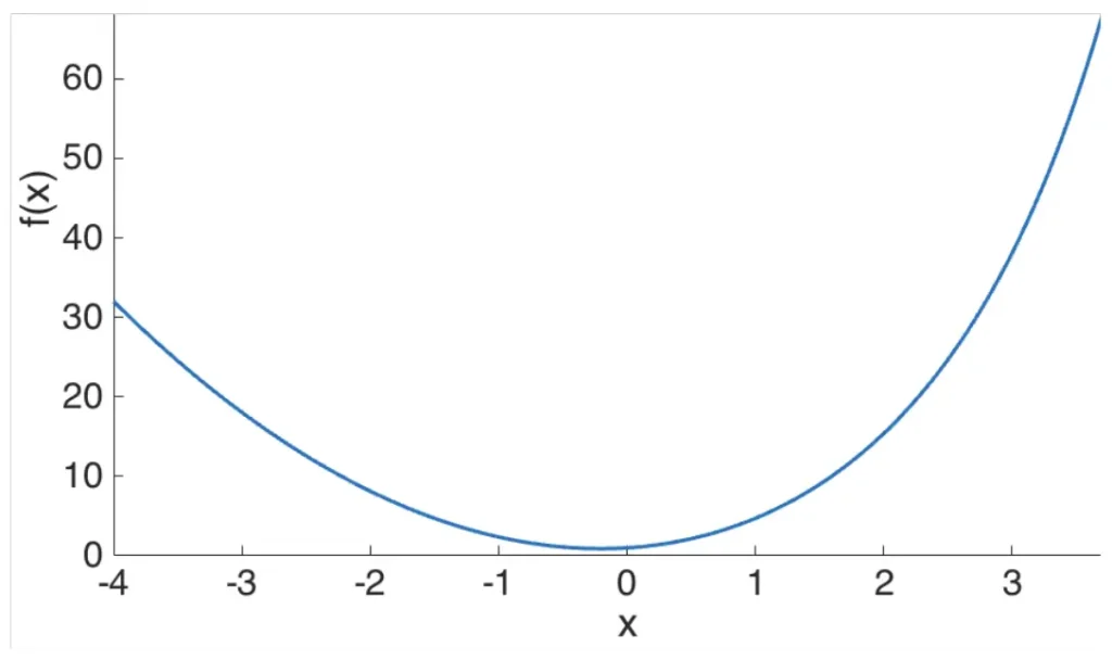
f(x) = e^x + 2 \cdot x^2
- Let’s find optimum of above function with brute force approach:
- Optimum is attained at with min value of .
- If we search the interval with step size , then we have to evaluate for times.
- This is so inefficient.
- Let’s find optimum of above function using adaptive grid search:
- We search interval with step size .
- At min point, we set new search interval as and we divide the step size by .
- We repeat this process until min point does not change then a tolerance value .
- This approach is times better than brute force approach.
- Can we do better ?
Local Minimizer
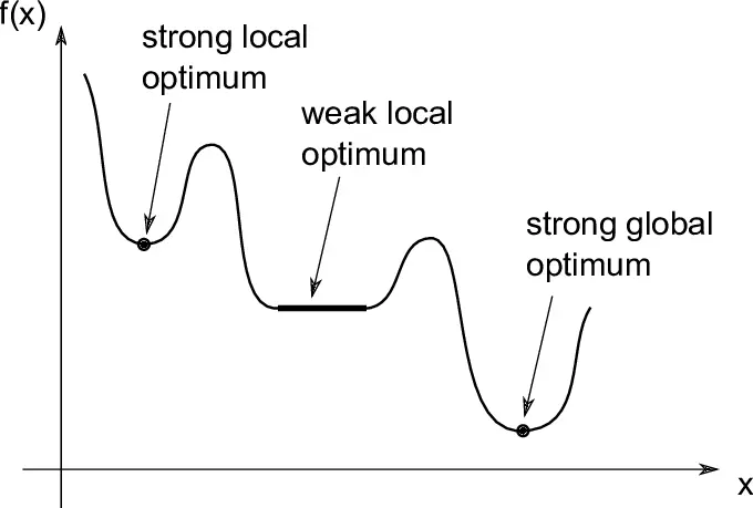
Local minimizer is a point that achieves the smallest value of in its neighbourhood.
- A point x is weak local minimizer if there is a neighbourhood of x such that
f(x^*) \leq f(x)
- A point x is strict (strong) minimizer if there is a neighbourhood of x such that
f(x^*) < f(x)
- For the constant value , every point of x is a weak local minimizer.
- For the function has a strict local minimizer at .
- To sum up, the formal definition is .
- There will be too much local minimas and we cannot know whether we are in global or not.
Vector Derivatives
- First order derivative = Gradient.
- Second order derivative = Hessian.
The function is given by:
f(x) = x_1 x_2 + 2x_1^2 - x_3
The vector x is:
x = \begin{bmatrix} x_1 \\ x_2 \\ x_3 \end{bmatrix}The gradient of is:
\nabla f(x) = \begin{bmatrix} \frac{\partial f(x)}{\partial x_1} \\ \frac{\partial f(x)}{\partial x_2} \\ \frac{\partial f(x)}{\partial x_3} \end{bmatrix}By calculating the partial derivatives, the gradient is:
\nabla f(x) = \begin{bmatrix} x_2 + 4x_1 \\ x_1 \\ -1 \end{bmatrix}The Hessian matrix ( H ) is defined as:
H = \nabla^2 f(x) =
\begin{bmatrix}
\frac{\partial^2 f(x)}{\partial x_1^2} & \frac{\partial^2 f(x)}{\partial x_1 \partial x_2} & \frac{\partial^2 f(x)}{\partial x_1 \partial x_3} \\
\frac{\partial^2 f(x)}{\partial x_2 \partial x_1} & \frac{\partial^2 f(x)}{\partial x_2^2} & \frac{\partial^2 f(x)}{\partial x_2 \partial x_3} \\
\frac{\partial^2 f(x)}{\partial x_3 \partial x_1} & \frac{\partial^2 f(x)}{\partial x_3 \partial x_2} & \frac{\partial^2 f(x)}{\partial x_3^2}
\end{bmatrix}
Observe that:
\frac{\partial^2 f(x)}{\partial x_1 \partial x_2} = \frac{\partial^2 f(x)}{\partial x_2 \partial x_1}\frac{\partial^2 f(x)}{\partial x_1 \partial x_3} = \frac{\partial^2 f(x)}{\partial x_3 \partial x_1}\frac{\partial^2 f(x)}{\partial x_2 \partial x_3} = \frac{\partial^2 f(x)}{\partial x_3 \partial x_2}Example: The function is given by:
f(x) = x_1^2 + 2x_2^2 - 3x_1 x_2The vector x is:
x = \begin{bmatrix} x_1 \\ x_2 \end{bmatrix}The gradient is:
\nabla f(x) = \begin{bmatrix} \frac{\partial f(x)}{\partial x_1} \\ \frac{\partial f(x)}{\partial x_2} \end{bmatrix} = \begin{bmatrix} 2x_1 - 3x_2 \\ 4x_2 - 3x_1 \end{bmatrix}The Hessian matrix is:
\nabla^2 f(x) = \begin{bmatrix} \frac{\partial^2 f(x)}{\partial x_1^2} & \frac{\partial^2 f(x)}{\partial x_1 \partial x_2} \\ \frac{\partial^2 f(x)}{\partial x_2 \partial x_1} & \frac{\partial^2 f(x)}{\partial x_2^2} \end{bmatrix} = \begin{bmatrix} 2 & -3 \\ -3 & 4 \end{bmatrix}
Taylor’s Theorem
First order Taylor expansion:
f(x + p) = f(x)
Second order Taylor expansion:
f(x + p) = f(x) + \nabla f(x + tp)^T p
Quadratic Taylor expansion:
f(x + p) = f(x) + \nabla f(x)^T p + \frac{1}{2} p^T \nabla^2 f(x + tp) pWhere x is variable, p is direction and
Example: Let’s use the Taylor theorem to approximate the function around .
f(x) \approx f(0) + f'(0)x + \frac{f''(0)}{2!}x^2 + \cdots + \frac{f^{(n)}(0)}{n!}x^nf(0) = 1f'(x) = e^x \Rightarrow f'(0) = 1f''(x) = e^x \Rightarrow f''(0) = 1e^x \approx 1 + x + \frac{x^2}{2!} + \frac{x^3}{3!} + \cdotsFor example, let’s approximate :
e^{0.1} \approx 1 + 0.1 + \frac{(0.1)^2}{2} = 1 + 0.1 + 0.005 = 1.105
Necessary Conditions
\nabla f(x^*) = 0
We call x* as stationary point if it gives above equality. Any local optimum must be stationary point.
Example: Find the stationary point of
f(x) = e^x - 4 \cdot x\nabla f(x^*) = e^x - 4e^x - 4 = 0 \rightarrow x^* = log(4)
Note: Gradient direction is always directed to increasing direction
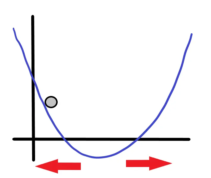
Let’s proof the with proof by contradiction:
- Assume that .
- Define vector .
- If we multiply with , we get .
- Because is continuous near , .
- For any , we have a Taylor theorem that .
- We showed that is negative.
- Therefore for all .
- But this is a contradiction because by definition is the lowest point.
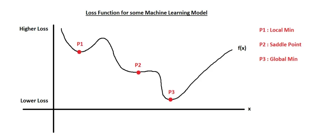
If we take derivative of these 3 points, all of them gives us 0, so how can we seperate them?
\nabla f(x^*) = 0
We can use second derivative:
- If , İt is minima.
- If , it is maxima.
- , then f is positive semidefinite.
- If , no conclusion at x (min, max or saddle point).
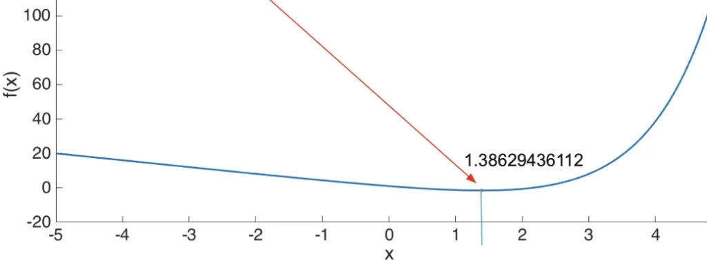
Example: For example, in above example the second derivative is
\nabla^2 f(x^*) = e^{\log(4)} = 4 > 0which is a local minimum.
Convexity
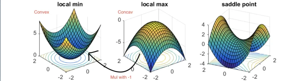
- Sum of convex functions is also convex function.
- In convex functions, local min is also global min.
Example: Linear Regression
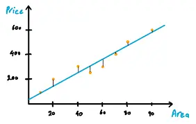
Suppose we have a function , and we want to fit a line to data. We need to minimize total distance between dots and the line.
- Each distance is , where is the estimated (on the line) value and is the real value.
- So our cost function is:
J = \sum_{i=1}^{n} (\hat{y}_i - y_i)^2 = \sum_{i=1}^{n} r_i^2 = \sum_{i=1}^{n} (m \cdot x_i + b - y_i)^2- So we need to minimize J with respect to m and b:
J = \frac{1}{2} \sum_{i=1}^{n} (\hat{y_i} - y_i)^2\nabla J = \begin{bmatrix} \frac{\partial J}{\partial m} \\ \frac{\partial J}{\partial b} \end{bmatrix} = \begin{bmatrix} 0 \\ 0 \end{bmatrix}\frac{\partial J}{\partial m} = \frac{1}{2} \sum \frac{\partial}{\partial m} (\hat{y_i} - y_i)^2 = 0\sum (\hat{y_i} - y_i)(y_i)' = 0- If we simplify further:
\sum_{i=1}^{n} (mx_i + b - y_i)x_i = 0\sum_{i=1}^{n} (mx_i^2 + bx_i - x_i y_i) = 0\sum_{i=1}^{n} mx_i^2 + \sum_{i=1}^{n} bx_i - \sum_{i=1}^{n} x_i y_i = 0m \sum_{i=1}^{n} x_i^2 = \sum_{i=1}^{n} x_i y_i - b \sum_{i=1}^{n} x_im = \frac{\sum_{i=1}^{n} x_i y_i - b x_i}{\sum_{i=1}^{n} x_i^2}- We can do this also for finding b, then we get the our solution.
- We can write a code for this:
Initialize and
For to :
End For- And we finally get the m and b, and also we find the best line as .
In some non-linear cases, we cannot get the .